How video compression takes advantage of your eyes

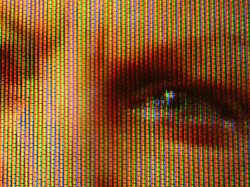
The real world inherently presents an analog, continuous stream of visual information. Due to how modern electronics works, we need to encode these analog information into digital ones. As any visual representation in the field of images and videos has humans as ultimate consumers, the solutions are equally shaped by the technological state-of-the-art and the limitations and peculiarities of the Human Visual System. The Human Visual System is the human’s visual interface with the surrounding world and having a thorough knowledge of it allows us to focus our effort on aspects that can actually be perceived by our eyes rather than ones that go unnoticed.

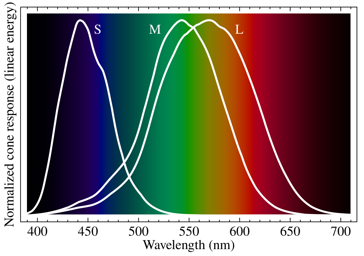
An example of how technology evolved in accordance to the human eyes are the color spaces that we use to digitally represent colours. The most common color spaces: sRGB, Rec. 709 and Rec. 2020 are all additive color models where the primary colours red, green and blue are summed together to obtain any other color. The choice to use red, green and blue as primary colours is not by chance but is determined by the physical characteristics of the Human Visual System. As originally described by the Young–Helmholtz theory Human eyes are said to be trichromats which means that they posses three independent channels for conveying color information. Three cells respond most to yellow, green, and violet and the reason we use RGB is because these frequencies can be efficiently stimulated using Red, Green and Blue. These cells are usually identified using respectively the letters S, M and L. The way the wavelength and the cell’s perception work is visible below.

Left: in the RGB color space, any color is created by combining different intensities of Red, Green and Blue. Right: the sensitivity of human cone cells to different frequencies of colors. Image source: Wikipedia.

Cone cell sensitivity — Left: in the RGB color space, any color is created by combining different intensities of Red, Green and Blue. Right: the sensitivity of human cone cells to different frequencies of colors. Image source: Wikipedia.

When examining carefully the video and photo standards it’s easy to come to appreciate how design decisions that seem totally arbitrary at first glance are in reality dictated by how the human’s eyes and nervous system work. Video Compression Algorithms, Video Management System and video formats are no exception and to understand the state-of-the-art in these fields we also need to understand the Human Visual System internals. A gap exists between the human’s perception of reality and the physical reality: modern compression algorithms exploit this gap to dramatically reduce the amount of data that needs to be transmitted to convey a certain information. The following sections are going to analyze aspects of the Human Visual System which profoundly impact how the previously mentioned field evolved.

This post is adapted from the background chapters of my master thesis where I used video compression metadata for efficient motion detection using machine learning.

Human Perception of Luminance and Chrominance

In the field of digital videos and photos, the most used color space is YCbCr. Essentially, YCbCr is a way to encode an RGB color in a way that is more efficient for the Human Visual System.

As the name suggests, the YCbCr color space is composed of three distinct components:

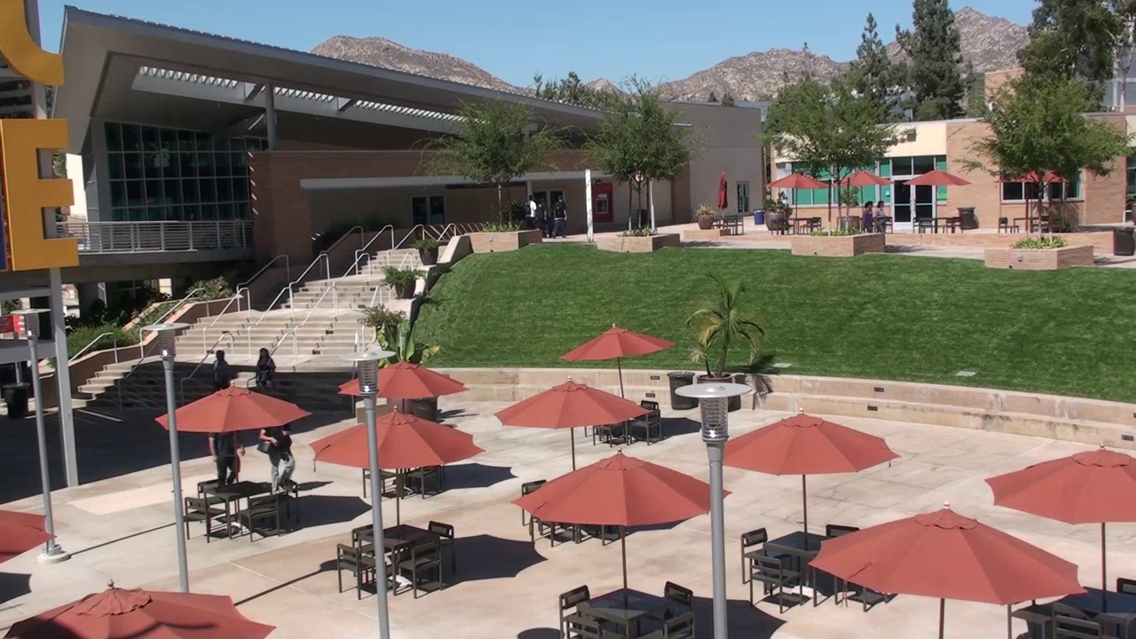
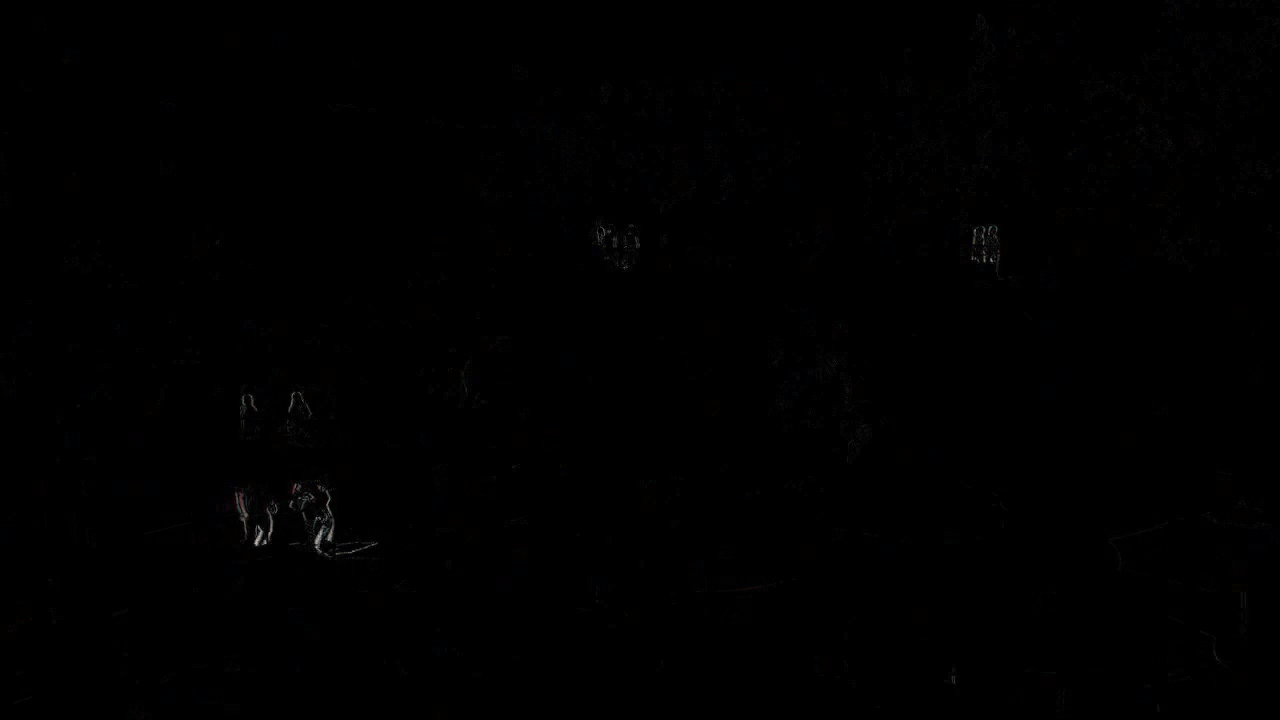
Y: represents the luminance. This is the weighted sum of the individual components of RGB and is similar to the black and white version of the image being encoded. In the ITU601, the Y is calculated using the formula: Y = 0.299 × R + 0.587 × G + 0.114 × B The weight assigned to each color, maps how sensitive the Human Visual System is to that color.
Cb: represents the difference between the blue component and the luminance. When it’s positive, the color leans towards blue. When it’s negative it leans towards yellow. Cb is computed as: Cb = 0.564 × (B - Y) + 128
Cr: represents the difference between the red component and the luminance. Cr is computed as: Cr = 0.713 × (R - Y) + 128

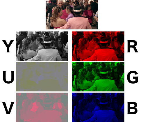
YCbCr vs RGB — Left: the Y, Cb and Cr channels of the top image. Right: the R, G and B channels of the right image. Image adapted from gnome.org.

The key difference between RGB and YCbCr is that in RGB, both luminance and chrominance information are distributed across all three channels, while YCbCr separates these components: luminance is entirely conveyed in the Y channel and chrominance in the Cb and Cr channels. This is, once again, dictated by the way the Human Visual System perceives the physical world. In particular, chrominance and luminance, are perceived using different kind of photoreceptors and the ones responsible for the chrominance are scarcer than the ones responsible for the perception of the chrominance. As a consequence, humans are more sensitive to variation of brightness rather than variation of color.

Under these circumstances, it is not beneficial to encode the same amount of information for chrominance and luminance as in RGB. Empirically, it is possible to see from the image above how in RGB the visual information are evenly spread among all the three channels while for YCbCr, the Y channel conveys much more visual information than Cb and Cr. By having the luminance and the chrominance in different channels, it is possible to encode the two features at different levels of detail. This is known as Chroma Subsampling. The different combinations of Chroma Subsampling are expressed as a three components ratio J:a:b where these components represent:

J: is the horizontal sampling reference window.
a: represents the number of samples in the first row of J pixels.
b: represents the number of samples in the second row of J pixels.

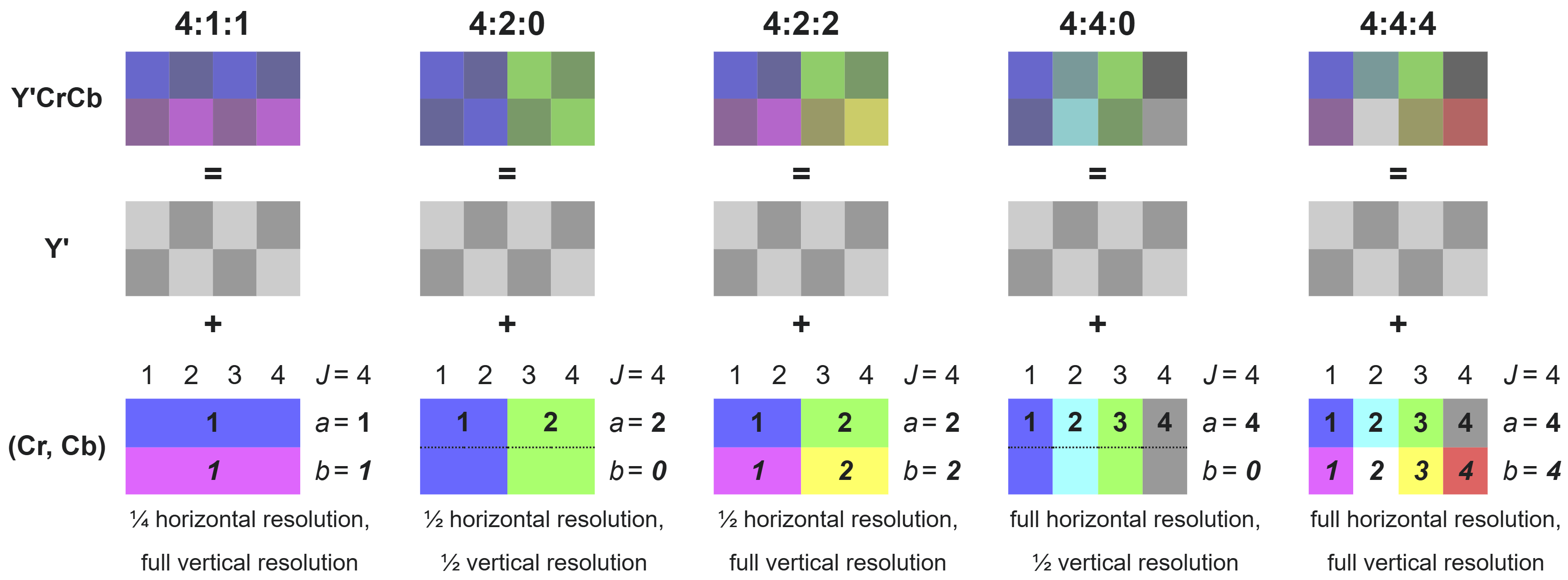
When using a 4:2:2 Chroma Subsampling, we obtain a bandwidth reduction of one third when compared to RGB with no impact on visual perception. Even when more aggressive subsampling are used, like the 4:2:0 subsampling used below, there is minimal impact on perceived visual quality by the Human Visual System while reducing the bandwidth up to half of what would be needed when using RGB.

Human Perception of Image Frequency

Like sounds, images also have frequencies and it is another crucial aspect of image compression.

In the domain of sounds, the frequency represents the variation in air pressure over time. Similarly, for images the frequency is the variation in pixel color and intensity over the space of the image.

As is possible to appreciate in the image below, in the space of the same image is possible to find regions that are high frequency and regions that are low frequency. Low frequencies regions are solid or smooth gradients where the pixel change is non-existent or very limited over space. High frequency regions are fine textures, texts or static noise and any other case where pixel values change rapidly.

As described above for what concerns Chrominance and Luminance, the Human Visual System also has varied frequency sensitivity. Frequency in images is measured in cycles per degree and frequencies that are considered low (below 0.1 cpp) or high (over 0.25 cpp) are difficult to perceive.

Both JPEG, H.264 and other lossy visual compression algorithms use this characteristic of the Human Visual System to reduce the amount of information encoded, and therefore the amount of bytes needed to represent it, while resulting in a perceived loss of quality that is minimal or absent.

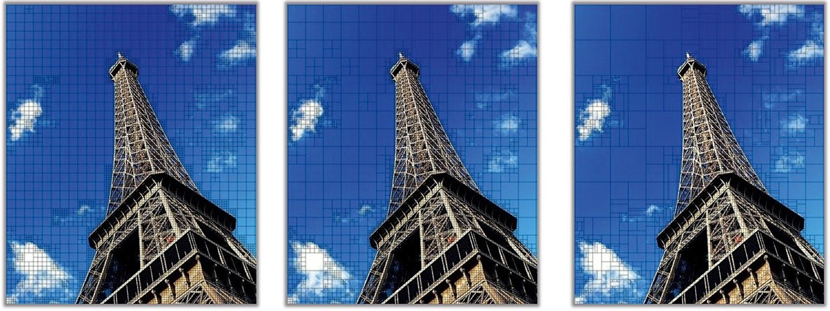
An example of a compression technique which leverages this characteristic of the Human Visual System is H.264’s Discrete Cosine Transformation (DCT). In the image below it is possible to see the same image with different level compressed using H.264 and various DCT coefficient. This images, are a perfect example of how the Human Visual System sensitivity to high frequencies is very low. Without zooming in the images, it is difficult to notice the difference between a low DCT coefficient and a high DCT coefficient. The difference becomes obvious only when we perform a severe zooming in a high frequency region of the image.

Reducing the high frequency detail of an image enable other optimization which ultimately result in dramatic size reduction of the image. In the image below we can empirically observe how even when shedding almost 60% of the image weight (in the DCT 28 column) the difference to the naked eye is still minimal.

Video Compression Algorithms

Several compression techniques have been developed with the ultimate goal of reducing the amount of bits needed to represent a video. The fundamental reason that drove the demand and consequently the effort to develop compression algorithms mainly comes from the sheer volume that uncompressed videos occupy.

A single uncompressed 1080p frame has a width of 1920 pixels and an height of 1080 pixels. Given that in the True Color standard each color channel (respectively Red, Green and Blue) is encoded using an 8 bit integer, a single uncompressed frame of this format requires 6.22 Megabytes. The industry standard in the field of Video Management Systems is to have videos with 30 fps. This means that a single minute of an uncompressed 1080p True Color video would require 11.2 Gigabytes.

As the number of pixels has a growth factor of O(n²) where n represent the scaling factor of the resolution, to represent the same video using a 4K resolution, 44.4 Gigabytes would be required.

As already introduced in the previous sections, most of the information contained in the uncompressed video, are way beyond what the Human Visual System can perceive and we can get rid of some of these information with minimal or no loss of perceived quality.

Today, the industry standard is H.264 and it’s successive iterations: H.265 and H.266. All the H.26x family of algorithms, are based on two principles:

Reducing the amount of information
Reducing the information redundancies

An example of the first is given in the chrominance and frequency sections above. An example of the second is run-length encoding (RLE): if we have a region of one thousand pixels of the same color, instead of writing one entry for each pixel we can just write the information once followed by how many times it needs to be repeated. An example of RLE is displayed below. RLE is not part of the techniques applied by H.264 nor by its successive iterations but other techniques which share the same principle are actually used. When redundancies are eliminated within the same frame, This is known as spatial compression while when it is applied across frames it takes the name of temporal compression. Several examples from H.264 of spatial and temporal compression are described in the next sections.

a  a  a  b  c  c  c  c
        │
        ▼
a  3  b  1  c  4

Run-length encoding is an example of a spatial compression technique. Instead of writing the same information multiple times in a row, the information is written only once and the number of times it is repeated is specified.

Discrete Cosine Transformation

The DCT is the most widely used linear transform in the field of lossy data compression. It can be adapted to represent an arbitrary piece of information as the sum of cosine function. Although it is widely used for many digital content, what makes it particularly efficient in the field of image and video compression is that: in general most of the information is very skewed in a few low frequencies.

Rather than applying the transformation to the image as a whole, in JPEG and in H.26x it is applied on sub-blocks of the image. In H.264, this is applied either on 4x4 or 8x8 sub-macroblocks. This is known as blocked DCT.

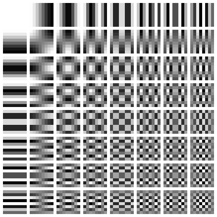
DCT components — Visualization of the basic components used in an 8x8 DCT transformation. The blocks in the matrix have increasing vertical frequency from left to right and higher horizontal frequency from top to bottom. Source: yasoob.me

Any 8x8 pixel block can be encoded in an 8x8 DCT coefficients matrix where each element corresponds to the coefficients associated with each block of a 2D DCT basic function. When applying the second DCT transform using an 8x8 DCT basic function like the one reported above, a matrix of coefficients is the output. An example output of this process is displayed below, where four different 8x8 blocks and their corresponding coefficients as calculated by the second DCT transform.

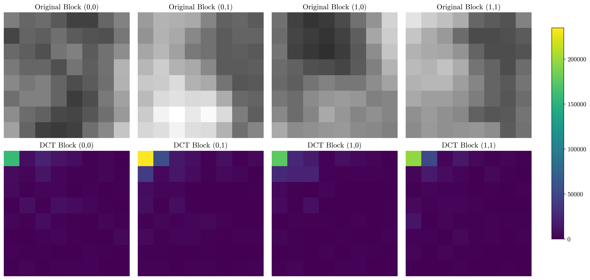
DCT blocks — In the upper row, four arbitrary 8x8 pixels blocks. In the bottom row, the corresponding DCT coefficient when applying an H.264 style second DCT.

In the image above, the high compression properties of DCT are empirically visible. No matter what are the values that needs to be encoded, the magnitude of the coefficients will always be highly skewed towards the low frequencies (top-left corner of the matrix) while the rest of the coefficients will be very close to 0.

As low coefficients mean that it contributes less to the final image, and as the Human Visual System is not sensitive to high frequencies anyway (as discussed earlier), DCT does not just allow to encode complex patterns in a few coefficient, we can also eliminate some of them without any noticeable effect on the final image.

Some of the values are discarded in the quantization stage, where the initial DCT coefficients are multiplied with a quantization matrix and then rounded to the nearest integer.

Although DCT is inherently lossless, the quantization stage that is usually applied after the transform makes it lossy. The quantization matrix is what determines the amount of information that is lost. By using quantization matrix that results in lighter images, more coefficients are quantized to zero. In the image below, the DCT coefficients are quantized using H.264’s highest compression quantization matrix.

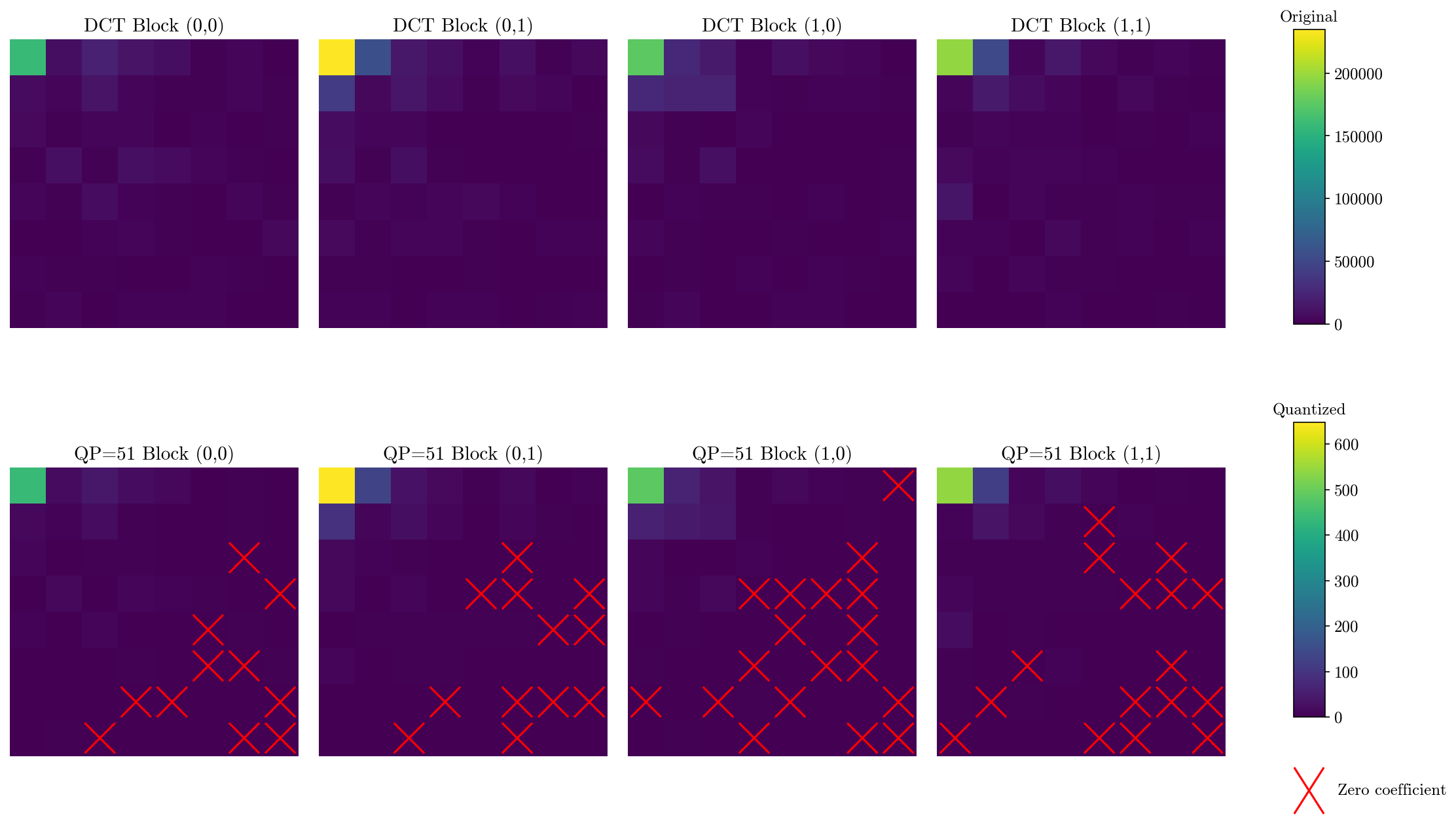
DCT quantization — In the upper row, DCT coefficients as in the previous figure. In the bottom row, the same coefficients after applying the highest compression quantization matrix from H.264. The coefficients that are zero are highlighted by a red cross on the corresponding cell. A lot of the coefficients in the bottom left corner of the matrix are quantized to zero.

The quantized coefficients are then encoded in a one dimension array of coefficients using a zig-zag pattern. As after quantization the bottom left of the matrix usually has several zero values this also makes the quantized coefficients the perfect candidate for another spatial compression technique which is called entropy coding and is further discussed below.

Frame Partitioning

Frames are subdivided in partitions. Although these are not in itself a spatial or temporal compression technique, it is a building block which is fundamental to several other compression techniques like Motion Compensation which is discussed in depth later.

Processing all the pixels in a frame together would have not been practical nor efficient also in old coded standard like H.264, but this is especially evident with the last iteration, H.266, which supports video resolutions up to 8k (7680x4320 pixels (a total of 33.2 million pixels per frame)). Macroblocks are a natural solution to this obstacle.

Processing small blocks is a better solution for modern CPU architectures for two reason. The first reason is that modern processors have small multilevel caches which are extremely faster than the rest of the memory. Processing smaller chunks of data allows them to fit in the cache at all time. Avoiding accessing the lowest levels of the memory hierarchy which ultimately results in more than linear speed up. In fact, macroblocks are extremely similar to another technique widely used in numerical methods and in High Performance Computing (HPC) which is blocking. The other reason is that, once divided, these smaller blocks can be processed independently. As modern CPUs have core counts that are approaching the hundreds and as GPUs have several thousands cores enabling parallelism allows leveraging all the resources that modern hardware provides.

Codec partitions — From left to right, the subdivision in partitions of H.264, H.265 and H.266. With each new codec release, both the maximum partitions size and the variety of shapes that macroblocks can take have progressively increased.

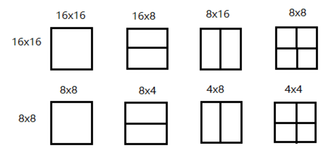
As it is possible to see in the image above, the trend in the H.26x codes is to have blocks that are increasingly bigger and with more varied and complex shapes. In H.264, the blocks are called macroblocks and the maximum size is 16x16 pixels. A 16x16 pixels macroblock can be additionally subdivided up to 4x4 pixels sub-macroblocks.

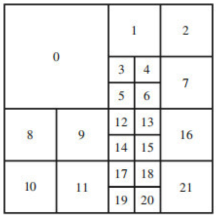
H.264 macroblocks — All the possible macroblocks in H.264. Adapted from: blog.csdn.net

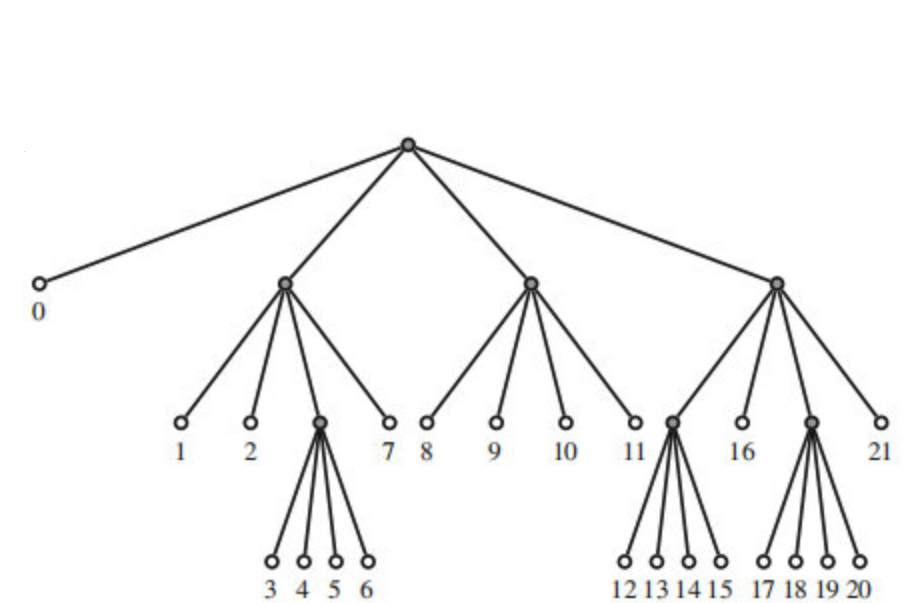
In H.265 and H.266, the macroblocks are replaced by Coding Tree Unit (CTU) which are a much more complex structure. The frame is once again entirely divided into squares of 64x64 pixels for H.265 and of 124x124 pixels for H.266. Each of these fixed size square is a CTU and each of them is associated with a Quad-Tree which keeps the information regarding the subdivision of the underlying level. The decoder can then choose to use a further quad tree if the underlying level is also partitioned or a termination node instead. A quad-tree and the resulting CTU subdivision are presented below.

In H.266, in addition to bigger CTU partition, also more complex shapes are supported which results in the use of a Quad-Tree plus Multi-Type Tree (QTMT). At any level of the tree, the decoder can choose among different trees depending on the way the block is further subdivided. The possible trees are:

Quad-tree: when the deeper level is divided into four sub blocks.
Ternary-tree: when the deeper level is divided in three sub blocks.
Binary-tree: when the deeper level is divided into two sub blocks.
Termination node: when the block is the deepest level.

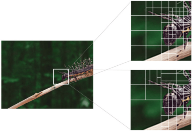
A visual comparison of the different partitioning results between H.265 and H.266 is visible below. Thanks to the bigger maximum CTU size and thanks to more complex partitioning trees, the results are substantially different.

H.265 vs H.266 — On the upper right, the H.265 partitioning of a macroblock. On the lower right, the H.266 partitioning of the same block.

Having such complex frame partitioning is pivotal for Motion Compensation (discussed in depth later) but also for more efficient DCT.

From the images above it is possible to notice that featureless sections of the image are characterized by bigger CTU or macroblocks while regions which contains more features are characterized by a more complex and finer grain partitioning. This is because lower frequencies areas are easier to describe and therefore bigger regions can be encoded with less data. At the same time, high frequency regions are more difficult to encode using DCT and therefore, smaller blocks are required.

Higher and more adaptable frame partitioning results in higher encoding efficiencies and bandwidth saving.

Beside DCT encoding, having more adaptable CTU also makes tracking the motion of objects across frames easier and therefore results in higher savings thanks to motion compensation.

This plays a big role in the increased bandwidth efficiency between H.264 and H.266. On the other hand, it also results in a higher complexity (the H.264 specification is half the length of the H.266 specification) and higher computational complexity (although partially offset by better accommodating parallelism).

Entropy Coding

Entropy coding is a compression technique which works by mapping an alphabet to an encoding and assigns shorter code words to more frequently occurring symbols and longer code words to less frequent ones. This method uses the statistical properties of information to reduce redundancy, allowing the most common data elements to be represented with the fewest bits.

A practical example of how entropy coding works is found in the morse alphabet. As the most common letter in English, Samuel Morse assigned it the shortest possible code: a single dot “.”. At the same time, letters that are less frequent such as z and q have been assigned longer code, respectively “–.-“ and “–..”. This elegant distribution of code lengths mirrors the statistical frequency of each letter, ensuring messages could be transmitted with maximum efficiency and minimum time.

In H.264, H.265 and H.266, two entropy encoding: Context Adaptive Binary Arithmetic Coding (CABAC) and Context Adaptive Variable Length Coding (CAVLC) are used to encode the residuals using less bandwidth than if they were to be written in the stream as they are.

CABAC results in better compression when compared to CAVLC while also requiring higher computation. When these entropy encoding techniques are applied to the DCT coefficients after the quantization steps they results in a factor of 10 compression for quantization that still preserve good visual quality and a factor of 14 for the highest available quantization in H.264. Compared to CAVLC, CABAC achieves compression between 9-14% better than CABAC.

The explanation for such dramatic compression is to be attributed to the fact that the quantization step applied to the DCT coefficient, especially at higher level of quantization, results in several zeros in the coefficients, especially in the lower frequencies.

To make this concrete, consider a quantized 4×4 DCT coefficient block after zigzag scan:

X = [0, 3, -1, 0, 0, -1, 1, 0, 0, 0, 0, 0, 0, 0, 0, 0]

As we know that most probably, only the first coefficient will be non-zero and the following will be zeros, we have a variable, TotalCoeff = 4 which counts the number of coefficients. Then another variable counts trailing ones as they have special statistical properties that can be exploited for more efficient compression (TrailingOnes = 3). Once we have these two variables, we can encode them using a CAVLC encoding table. Our case could result, for instance, in the encoded value 0000100.

For the sign of the trailing ones (TrailingOnes_sign), we encode each trailing one with a 0 for positive and 1 for negative, resulting in 110 for our three trailing ones.

For the remaining non-trailing-one coefficients (3), we encode using a level prefix and suffix:

Level prefix = 001, Level suffix = 0, Encoded level = 0010

In addition to this, the total number of zero before the last non zero value is also encoded. In our example this is 100.

The complete CAVLC bitstream requires just 21 bits: 0000100 110 0010 111 1 01 1. Without CAVLC encoding, the 16 quantized coefficients would require 8 bits each, for a total of 126 bits. In this example CAVLC achieves a compression ratio of approximately 7:1.

Motion Compensation

Most of the time, two consecutive frame have very little difference. If both frames are entirely written in the video stream, a lot of information that are common to both both would be redundant. Eliminating these redundancies is the key idea behind temporal compression and motion compensation.

Original frame — On the left, a frame of a CCTV footage. On the right, the residual between the frame on the left and the following one. The black pixels represent no difference between the frame and the following one. The vast majority of the pixels are identical among the frames.

Frame difference — On the left, a frame of a CCTV footage. On the right, the residual between the frame on the left and the following one. The black pixels represent no difference between the frame and the following one. The vast majority of the pixels are identical among the frames.

To understand how this is implemented in H.264, several concepts need to be introduced. First of all, different kind of frames are used, namely I-Frames, P-Frames and B-Frames.

The I-Frames, also referenced as key frames, are frames where the entire image is encoded in the video stream. They are self-contained and do not require any other frame to be decoded.
P-Frames are frames which only encode the difference from a previous reference frame (typically an I-frame or another P-frame). They use motion compensation to predict content based on previously decoded frames, storing only motion vectors and residual differences.
B-Frames are bi-directionally predicted frames that reference both past and future frames. They achieve higher compression by choosing the optimal prediction from frames on either side temporally, making them efficient but requiring out-of-order decoding.

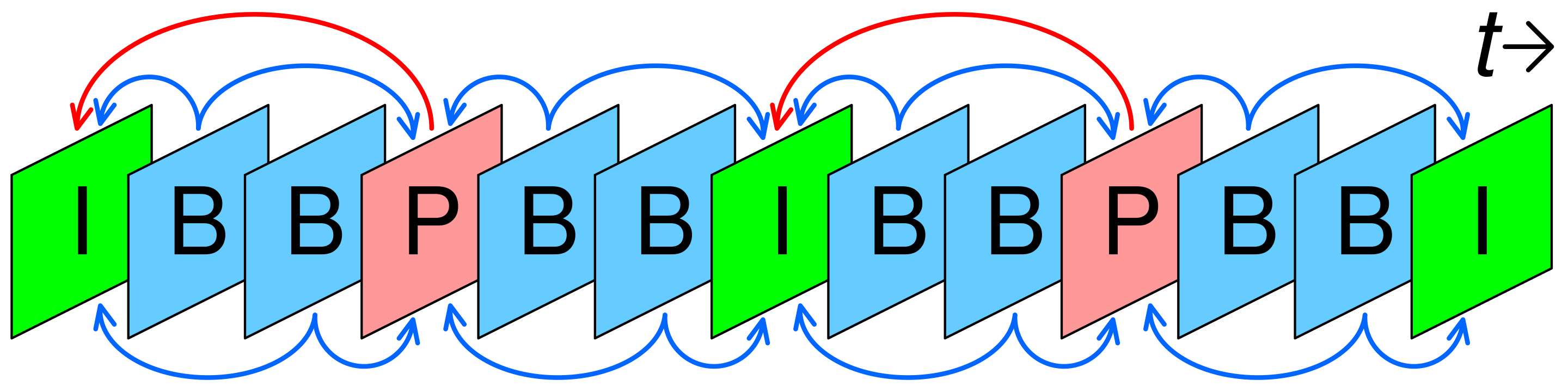
Frame types — In the H.264 standard and their successive iterations, the video stream is composed of interleaved I-Frames, P-Frames and B-Frames. The arrows represent the reference to preceding or following frames. Source: wikipedia.com

In H.264, the choice on how to interleave different kind of frames is entirely left to the encoder and is not defined by the H.264 standard. But, generally I-frames are found once every second. More severe compression might have a single I-Frame at the beginning of the stream and only rely on P-Frames for the entire video. I-Frames are the least efficient to encode, but, are also the only ones that are self-contained and can be decoded without any other information from other frames. If we want to decode an arbitrary P-Frame we first need to decode all the frames between the last I-Frame and the frame we want to decode. As especially when used in context where data can be lost during a network transmission, having more I-Frames is better for reliability.

Conclusion

If I picked your interest, go read my full thesis.